Clustering Music Genres with Machine Learning
Clustering is a machine learning technique to group data points characterized by specific features. Clustering music genres is a task of grouping music based on the similarities in their audio characteristics. If you want to learn how to perform clustering analysis on music genres, this article is for you. In this article, I will take you through the task of clustering music genres with machine learning using Python.
Clustering Music Genres (Problem Statement)
Every person has a different taste in music. We cannot identify what kind of music does a person likes by just knowing about their lifestyle, hobbies, or profession. So it is difficult for music streaming applications to recommend music to a person. But if we know what kind of songs a person listens to daily, we can find similarities in all the music files and recommend similar music to the person.
That is where the cluster analysis of music genres comes in. Here you are given a dataset of popular songs on Spotify, which contains artists and music names with all audio characteristics of each music. Your goal is to group music genres based on similarities in their audio characteristics.
You can download the dataset from here.
Clustering Music Genres using Python
I hope you have understood the problem statement mentioned above on clustering music genres with machine learning. Now let’s start with this task by importing the necessary Python libraries and the dataset:
import pandas as pd
import numpy as np
from sklearn import cluster

data = pd.read_csv("Spotify-2000.csv")
print(data.head())
Index Title Artist Top Genre \ 0 1 Sunrise Norah Jones adult standards 1 2 Black Night Deep Purple album rock 2 3 Clint Eastwood Gorillaz alternative hip hop 3 4 The Pretender Foo Fighters alternative metal 4 5 Waitin' On A Sunny Day Bruce Springsteen classic rock Year Beats Per Minute (BPM) Energy Danceability Loudness (dB) \ 0 2004 157 30 53 -14 1 2000 135 79 50 -11 2 2001 168 69 66 -9 3 2007 173 96 43 -4 4 2002 106 82 58 -5 Liveness Valence Length (Duration) Acousticness Speechiness Popularity 0 11 68 201 94 3 71 1 17 81 207 17 7 39 2 7 52 341 2 17 69 3 3 37 269 0 4 76 4 10 87 256 1 3 59
You can see all the columns of the dataset in the above output. It contains all the audio features of music that are enough to find similarities. Before moving forward, I will drop the index column, as it is of no use:
data = data.drop("Index", axis=1)Now let’s have a look at the correlation between all the audio features in the dataset:
print(data.corr()) Year Beats Per Minute (BPM) Energy \
Year 1.000000 0.012570 0.147235
Beats Per Minute (BPM) 0.012570 1.000000 0.156644
Energy 0.147235 0.156644 1.000000
Danceability 0.077493 -0.140602 0.139616
Loudness (dB) 0.343764 0.092927 0.735711
Liveness 0.019017 0.016256 0.174118
Valence -0.166163 0.059653 0.405175
Acousticness -0.132946 -0.122472 -0.665156
Speechiness 0.054097 0.085598 0.205865
Popularity -0.158962 -0.003181 0.103393
Danceability Loudness (dB) Liveness Valence \
Year 0.077493 0.343764 0.019017 -0.166163
Beats Per Minute (BPM) -0.140602 0.092927 0.016256 0.059653
Energy 0.139616 0.735711 0.174118 0.405175
Danceability 1.000000 0.044235 -0.103063 0.514564
Loudness (dB) 0.044235 1.000000 0.098257 0.147041
Liveness -0.103063 0.098257 1.000000 0.050667
Valence 0.514564 0.147041 0.050667 1.000000
Acousticness -0.135769 -0.451635 -0.046206 -0.239729
Speechiness 0.125229 0.125090 0.092594 0.107102
Popularity 0.144344 0.165527 -0.111978 0.095911
Acousticness Speechiness Popularity
Year -0.132946 0.054097 -0.158962
Beats Per Minute (BPM) -0.122472 0.085598 -0.003181
Energy -0.665156 0.205865 0.103393
Danceability -0.135769 0.125229 0.144344
Loudness (dB) -0.451635 0.125090 0.165527
Liveness -0.046206 0.092594 -0.111978
Valence -0.239729 0.107102 0.095911
Acousticness 1.000000 -0.098256 -0.087604
Speechiness -0.098256 1.000000 0.111689
Popularity -0.087604 0.111689 1.000000
Clustering Analysis of Audio Features
Now I will use the K-means clustering algorithm to find the similarities between all the audio features. Then I will add clusters in the dataset based on the similarities we found. So let’s create a new dataset of all the audio characteristics and perform clustering analysis using the K-means clustering algorithm:
data2 = data[["Beats Per Minute (BPM)", "Loudness (dB)",
              "Liveness", "Valence", "Acousticness",
              "Speechiness"]]

from sklearn.preprocessing import MinMaxScaler
for i in data.columns:
    MinMaxScaler(i)

from sklearn.cluster import KMeans
kmeans = KMeans(n_clusters=10)
clusters = kmeans.fit_predict(data2)
Now I will add the clusters as predicted by the K-means clustering algorithm to the original dataset:
data["Music Segments"] = clusters
MinMaxScaler(data["Music Segments"])
data["Music Segments"] = data["Music Segments"].map({1: "Cluster 1", 2:
    "Cluster 2", 3: "Cluster 3", 4: "Cluster 4", 5: "Cluster 5",
    6: "Cluster 6", 7: "Cluster 7", 8: "Cluster 8",
    9: "Cluster 9", 10: "Cluster 10"})
Now let’s have a look at the dataset with clusters:
print(data.head())Title Artist Top Genre Year \ 0 Sunrise Norah Jones adult standards 2004 1 Black Night Deep Purple album rock 2000 2 Clint Eastwood Gorillaz alternative hip hop 2001 3 The Pretender Foo Fighters alternative metal 2007 4 Waitin' On A Sunny Day Bruce Springsteen classic rock 2002 Beats Per Minute (BPM) Energy Danceability Loudness (dB) Liveness \ 0 157 30 53 -14 11 1 135 79 50 -11 17 2 168 69 66 -9 7 3 173 96 43 -4 3 4 106 82 58 -5 10 Valence Length (Duration) Acousticness Speechiness Popularity \ 0 68 201 94 3 71 1 81 207 17 7 39 2 52 341 2 17 69 3 37 269 0 4 76 4 87 256 1 3 59 Music Segments 0 Cluster 1 1 Cluster 6 2 Cluster 2 3 Cluster 2 4 Cluster 3
Now let’s visualize the clusters based on some of the audio features:
import plotly.graph_objects as go
PLOT = go.Figure()
for i in list(data["Music Segments"].unique()):


    PLOT.add_trace(go.Scatter3d(x = data[data["Music Segments"]== i]['Beats Per Minute (BPM)'],
                                y = data[data["Music Segments"] == i]['Energy'],
                                z = data[data["Music Segments"] == i]['Danceability'],
                                mode = 'markers',marker_size = 6, marker_line_width = 1,
                                name = str(i)))
PLOT.update_traces(hovertemplate='Beats Per Minute (BPM): %{x} <br>Energy: %{y} <br>Danceability: %{z}')


PLOT.update_layout(width = 800, height = 800, autosize = True, showlegend = True,
                   scene = dict(xaxis=dict(title = 'Beats Per Minute (BPM)', titlefont_color = 'black'),
                                yaxis=dict(title = 'Energy', titlefont_color = 'black'),
                                zaxis=dict(title = 'Danceability', titlefont_color = 'black')),
                   font = dict(family = "Gilroy", color  = 'black', size = 12))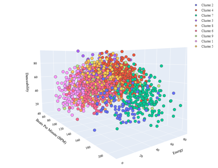
So this is how we can perform cluster analysis of music genres with machine learning.
Summary
So this is how you can perform cluster analysis of music genres with machine learning using Python. Clustering music genres is a task of grouping music based on the similarities in their audio features. I hope you liked this article on clustering music genres with machine learning. Feel free to ask valuable questions in the comments section below.