Currency Exchange Rate Forecasting using Python
The currency conversion rate or exchange rate is an important economic indicator affecting several sectors, such as import-export businesses, foreign investment and tourism. By analyzing past data and predicting future exchange rates, we can gain valuable insights to help stakeholders reduce risk, optimize currency conversions, and design effective financial strategies. So, if you want to know how to forecast currency exchange rates, this article is for you. In this article, I will take you through Currency Exchange Rate Forecasting using Python.
Currency Exchange Rate Forecasting: An Overview
Currency exchange rate forecasting means predicting future fluctuations in the value of one currency against another. It involves the use of historical data, economic indicators, and mathematical models to make accurate predictions about the direction and magnitude of exchange rate movements.
It helps individuals, businesses (such as import-export businesses, foreign investment and tourism), and financial institutions to anticipate market trends, mitigate risk, optimize currency conversions and plan strategic decisions.
To forecast exchange rates, we need historical data on the exchange rates between two currencies. I found an ideal dataset for this task. The dataset contains weekly exchange rates between INR and USD. You can download the dataset from here.
In the section below, I will take you through the task of Currency Exchange Rate Forecasting with Python using the INR – USD exchange rate data.
Currency Exchange Rate Forecasting using Python
I’ll start this task of Currency Exchange Rate Forecasting by importing the necessary Python libraries and the dataset:
import pandas as pd
import numpy as np
import matplotlib.pyplot as plt
import seaborn as sns
import plotly.express as px

data = pd.read_csv("INR-USD.csv")

print(data.head())
Date Open High Low Close Adj Close Volume 0 2003-12-01 45.709000 45.728001 45.449001 45.480000 45.480000 0.0 1 2003-12-08 45.474998 45.507999 45.352001 45.451000 45.451000 0.0 2 2003-12-15 45.450001 45.500000 45.332001 45.455002 45.455002 0.0 3 2003-12-22 45.417000 45.549000 45.296001 45.507999 45.507999 0.0 4 2003-12-29 45.439999 45.645000 45.421001 45.560001 45.560001 0.0
Let’s check if the dataset contains any missing values before moving forward:
print(data.isnull().sum())Date 0 Open 3 High 3 Low 3 Close 3 Adj Close 3 Volume 3 dtype: int64
The dataset has some missing values. Here’s how to remove them:
data = data.dropna()Now let’s have a look at the descriptive statistics of this dataset:
print(data.describe())Open High Low Close Adj Close Volume count 1013.000000 1013.000000 1013.000000 1013.000000 1013.000000 1013.0 mean 58.035208 58.506681 57.654706 58.056509 58.056509 0.0 std 12.614635 12.716632 12.565279 12.657407 12.657407 0.0 min 38.995998 39.334999 38.979000 39.044998 39.044998 0.0 25% 45.508999 45.775002 45.231998 45.498001 45.498001 0.0 50% 59.702999 60.342999 59.209999 59.840000 59.840000 0.0 75% 68.508499 69.099998 68.250000 68.538002 68.538002 0.0 max 82.917999 83.386002 82.563004 82.932999 82.932999 0.0
USD – INR Conversion Rate Analysis
As we are using the USD – INR conversion rates data, let’s analyze the conversion rates between both currencies over the years. I’ll start with a line chart showing the trend of conversion rates over the years:
figure = px.line(data, x="Date",
                 y="Close",
                 title='USD - INR Conversion Rate over the years')
figure.show()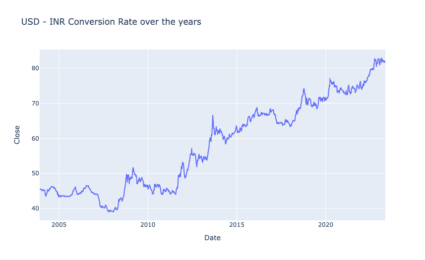
Now let’s add year and month columns in the data before moving forward:
data["Date"] = pd.to_datetime(data["Date"], format = '%Y-%m-%d')
data['Year'] = data['Date'].dt.year
data["Month"] = data["Date"].dt.month
print(data.head())
Date Open High Low Close Adj Close Volume \ 0 2003-12-01 45.709000 45.728001 45.449001 45.480000 45.480000 0.0 1 2003-12-08 45.474998 45.507999 45.352001 45.451000 45.451000 0.0 2 2003-12-15 45.450001 45.500000 45.332001 45.455002 45.455002 0.0 3 2003-12-22 45.417000 45.549000 45.296001 45.507999 45.507999 0.0 4 2003-12-29 45.439999 45.645000 45.421001 45.560001 45.560001 0.0 Year Month 0 2003 12 1 2003 12 2 2003 12 3 2003 12 4 2003 12
Now let’s have a look at the aggregated yearly growth of the conversion rates between INR and USD:
import plotly.graph_objs as go
import plotly.io as pio

# Calculate yearly growth
growth = data.groupby('Year').agg({'Close': lambda x: (x.iloc[-1]-x.iloc[0])/x.iloc[0]*100})

fig = go.Figure()
fig.add_trace(go.Bar(x=growth.index,
                     y=growth['Close'],
                     name='Yearly Growth'))

fig.update_layout(title="Yearly Growth of USD - INR Conversion Rate",
                  xaxis_title="Year",
                  yaxis_title="Growth (%)",
                  width=900,
                  height=600)

pio.show(fig)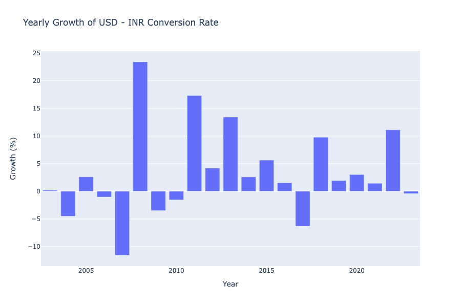
Now let’s have a look at the aggregated monthly growth of the conversion rates between INR and USD:
# Calculate monthly growth
data['Growth'] = data.groupby(['Year', 'Month'])['Close'].transform(lambda x: (x.iloc[-1] - x.iloc[0]) / x.iloc[0] * 100)

# Group data by Month and calculate average growth
grouped_data = data.groupby('Month').mean().reset_index()

fig = go.Figure()

fig.add_trace(go.Bar(
    x=grouped_data['Month'],
    y=grouped_data['Growth'],
    marker_color=grouped_data['Growth'],
    hovertemplate='Month: %{x}<br>Average Growth: %{y:.2f}%<extra></extra>'
))

fig.update_layout(
    title="Aggregated Monthly Growth of USD - INR Conversion Rate",
    xaxis_title="Month",
    yaxis_title="Average Growth (%)",
    width=900,
    height=600
)

pio.show(fig)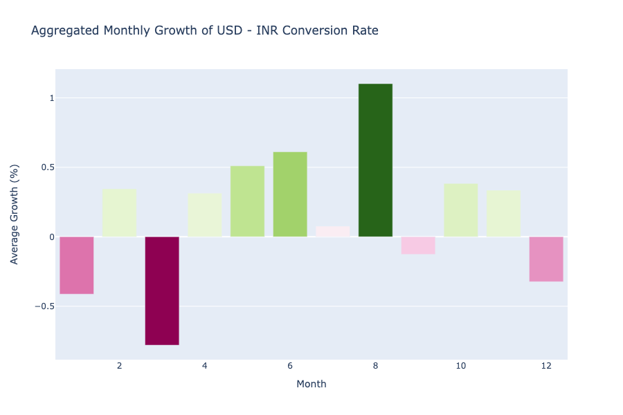
In the above graph, we can see that the value of USD always falls in January and March, while in the second quarter, USD becomes stronger against INR every year, the value of USD against INR peaks in August, but again falls in September, it rises again every year in the last quarter but falls again in December.
Forecasting Exchange Rates Using Time Series Forecasting
We will use time series forecasting to forecast exchange rates. To choose the most appropriate time series forecasting model, we need to perform seasonal decomposition, which will help us identify any recurring patterns, long-term trends, and random fluctuations present in the USD – INR exchange rate data:
from statsmodels.tsa.seasonal import seasonal_decompose
result = seasonal_decompose(data["Close"], model='multiplicative', period=24)
fig = plt.figure()
fig = result.plot()
fig.set_size_inches(8, 6)
fig.show()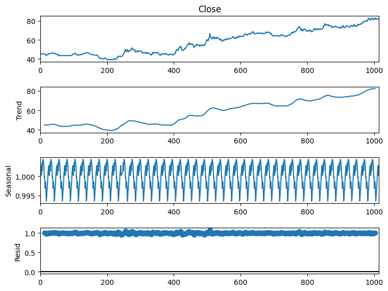
So we can see that there’s a seasonal pattern in this data. So SARIMA will be the most appropriate algorithm for this data. Before using SARIMA, we need to find p,d, and q values. Here, I will be using the pmdarima library to find these values. You can install this library in your Python environment by executing the command mentioned below:
- For terminal or command prompt: pip install pmdarima
- For Google Colab: !pip install pmdarima
Here’s how to find p,d, and q values using pmdarima:
from pmdarima.arima import auto_arima
model = auto_arima(data['Close'], seasonal=True, m=52, suppress_warnings=True)
print(model.order)
(2, 1, 0)
p, d, q = 2, 1, 0You can learn how to find these values manually without using pmdarima from here.
Now, here’s how to use SARIMA to train a model to forecast currency exchange rates:
from statsmodels.tsa.statespace.sarimax import SARIMAX
model = SARIMAX(data["Close"], order=(p, d, q),
                seasonal_order=(p, d, q, 52))
fitted = model.fit()
print(fitted.summary())
SARIMAX Results
==========================================================================================
Dep. Variable: Close No. Observations: 1013
Model: SARIMAX(2, 1, 0)x(2, 1, 0, 52) Log Likelihood -905.797
Date: Mon, 29 May 2023 AIC 1821.594
Time: 06:24:15 BIC 1845.929
Sample: 0 HQIC 1830.861
- 1013
Covariance Type: opg
==============================================================================
coef std err z P>|z| [0.025 0.975]
------------------------------------------------------------------------------
ar.L1 0.0313 0.026 1.193 0.233 -0.020 0.083
ar.L2 0.0643 0.026 2.481 0.013 0.013 0.115
ar.S.L52 -0.6358 0.026 -24.677 0.000 -0.686 -0.585
ar.S.L104 -0.3075 0.029 -10.602 0.000 -0.364 -0.251
sigma2 0.3767 0.013 28.481 0.000 0.351 0.403
===================================================================================
Ljung-Box (L1) (Q): 0.00 Jarque-Bera (JB): 86.43
Prob(Q): 0.99 Prob(JB): 0.00
Heteroskedasticity (H): 1.57 Skew: 0.06
Prob(H) (two-sided): 0.00 Kurtosis: 4.47
===================================================================================
Now here’s how to make predictions about future currency exchange rates:
predictions = fitted.predict(len(data), len(data)+60)
print(predictions)
1013 81.732807
1014 81.886990
1015 82.180319
1016 82.607754
1017 82.474242
...
1069 84.906873
1070 85.402528
1071 85.520223
1072 85.830554
1073 85.687360
Here’s how to visualize the forecasted results:
# Create figure
fig = go.Figure()

# Add training data line plot
fig.add_trace(go.Scatter(
    x=data.index,
    y=data['Close'],
    mode='lines',
    name='Training Data',
    line=dict(color='blue')
))

# Add predictions line plot
fig.add_trace(go.Scatter(
    x=predictions.index,
    y=predictions,
    mode='lines',
    name='Predictions',
    line=dict(color='green')
))

fig.update_layout(
    title="INR Rate - Training Data and Predictions",
    xaxis_title="Date",
    yaxis_title="Close",
    legend_title="Data",
    width=900,
    height=600
)

pio.show(fig)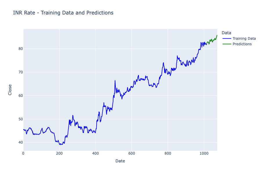
So this is how you can use time series forecasting for the task of Currency Exchange Rate Forecasting using Python.
Summary
Currency exchange rate forecasting means predicting future fluctuations in the value of one currency against another. It involves the use of historical data, economic indicators, and mathematical models to make accurate predictions about the direction and magnitude of exchange rate movements. I hope you liked this article on Currency Exchange Rate Forecasting using Python. Feel free to ask valuable questions in the comments section below.