Compare Multiple Machine Learning Models
The comparison of multiple Machine Learning models refers to training, evaluating, and analyzing the performance of different algorithms on the same dataset to identify which model performs best for a specific predictive task. So, if you want to learn how to train and compare multiple Machine Learning models, this article is for you. In this article, I’ll take you through how to train and compare multiple Machine Learning models for a regression problem using Python.
Compare Multiple Machine Learning Models: Process We Can Follow
By comparing multiple models, we aim to select the most effective algorithm that offers the optimal balance of accuracy, complexity, and performance for their specific problem. Below is the process we can follow for the task of comparing multiple Machine Learning models:
- Address missing values, remove duplicates, and correct errors in the dataset to ensure the quality of data fed into the models.
- Divide the dataset into training and testing sets, typically using a 70-30% or 80-20% split.
- Select a diverse set of models for comparison. It can include simple linear models, tree-based models, ensemble methods, and more advanced algorithms, depending on the problem’s complexity and data characteristics.
- Fit each selected model to the training data. It involves adjusting the model to learn from the features and the target variable in the training set.
- Use a set of metrics to evaluate each model’s performance on the test set.
- Compare the models based on the evaluation metrics, considering both their performance and computational efficiency.
I found an ideal dataset for this problem. You can download the dataset from here.
Train and Compare Multiple Machine Learning Models
Now, let’s get started with the task of training and comparing multiple Machine Learning models by importing the necessary Python libraries and the dataset:
import pandas as pd
data = pd.read_csv('Real_Estate.csv')

# display the first few rows
data_head = data.head()

print(data_head)
Transaction date House age Distance to the nearest MRT station \
0 2012-09-02 16:42:30.519336 13.3 4082.0150
1 2012-09-04 22:52:29.919544 35.5 274.0144
2 2012-09-05 01:10:52.349449 1.1 1978.6710
3 2012-09-05 13:26:01.189083 22.2 1055.0670
4 2012-09-06 08:29:47.910523 8.5 967.4000
Number of convenience stores Latitude Longitude \
0 8 25.007059 121.561694
1 2 25.012148 121.546990
2 10 25.003850 121.528336
3 5 24.962887 121.482178
4 6 25.011037 121.479946
House price of unit area
0 6.488673
1 24.970725
2 26.694267
3 38.091638
4 21.654710
print(data.info())<class 'pandas.core.frame.DataFrame'>
RangeIndex: 414 entries, 0 to 413
Data columns (total 7 columns):
# Column Non-Null Count Dtype
--- ------ -------------- -----
0 Transaction date 414 non-null object
1 House age 414 non-null float64
2 Distance to the nearest MRT station 414 non-null float64
3 Number of convenience stores 414 non-null int64
4 Latitude 414 non-null float64
5 Longitude 414 non-null float64
6 House price of unit area 414 non-null float64
dtypes: float64(5), int64(1), object(1)
memory usage: 22.8+ KB
None
The dataset consists of 414 entries and 7 columns, with no missing values. Here’s a brief overview of the columns:
- Transaction date: The date of the house sale (object type, which suggests it might need conversion or extraction of useful features like year, month, etc.).
- House age: The age of the house in years (float).
- Distance to the nearest MRT station: The distance to the nearest mass rapid transit station in meters (float).
- Number of convenience stores: The number of convenience stores in the living circle on foot (integer).
- Latitude: The geographic coordinate that specifies the north-south position (float).
- Longitude: The geographic coordinate that specifies the east-west position (float).
- House price of unit area: Price of the house per unit area (float), which is likely our target variable for prediction.
So, we are solving a regression problem here. In the next steps, we will preprocess the data and select regression models to find the best-performing model for our problem.
Data Preprocessing
Let’s start with the preprocessing steps. Below are the steps we will follow to preprocess our data:
- Since the transaction date is in a string format, we will convert it into a datetime object. We can then extract features such as the transaction year and month, which might be useful for the model.
- We’ll scale the continuous features to ensure they’re on a similar scale. It is particularly important for models like Support Vector Machines or K-nearest neighbours, which are sensitive to the scale of input features.
- We’ll split the dataset into a training set and a testing set. A common practice is to use 80% of the data for training and 20% for testing.
Let’s implement these preprocessing steps:
from sklearn.model_selection import train_test_split
from sklearn.preprocessing import StandardScaler
import datetime

# convert "Transaction date" to datetime and extract year and month
data['Transaction date'] = pd.to_datetime(data['Transaction date'])
data['Transaction year'] = data['Transaction date'].dt.year
data['Transaction month'] = data['Transaction date'].dt.month

# drop the original "Transaction date" as we've extracted relevant features
data = data.drop(columns=['Transaction date'])

# define features and target variable
X = data.drop('House price of unit area', axis=1)
y = data['House price of unit area']

# split the data into training and testing sets
X_train, X_test, y_train, y_test = train_test_split(X, y, test_size=0.2, random_state=42)

# scale the features
scaler = StandardScaler()
X_train_scaled = scaler.fit_transform(X_train)
X_test_scaled = scaler.transform(X_test)

X_train_scaled.shape
(331, 7)
X_test_scaled.shape(83, 7)
Model Training and Comparison
Now, we’ll proceed with training multiple models and comparing their performance. We’ll start with a few commonly used models for regression tasks:
- Linear Regression: A good baseline model for regression tasks.
- Decision Tree Regressor: To see how a simple tree-based model performs.
- Random Forest Regressor: An ensemble method to improve upon the decision tree’s performance.
- Gradient Boosting Regressor: Another powerful ensemble method for regression.
We’ll train each model using the training data and evaluate their performance on the test set using Mean Absolute Error (MAE) and R-squared (R²) as metrics. These metrics will help us understand both the average error of the predictions and how well the model explains the variance in the target variable.
Let’s start with training these models and comparing their performance:
from sklearn.linear_model import LinearRegression
from sklearn.tree import DecisionTreeRegressor
from sklearn.ensemble import RandomForestRegressor, GradientBoostingRegressor
from sklearn.metrics import mean_absolute_error, r2_score

# initialize the models
models = {
    "Linear Regression": LinearRegression(),
    "Decision Tree": DecisionTreeRegressor(random_state=42),
    "Random Forest": RandomForestRegressor(random_state=42),
    "Gradient Boosting": GradientBoostingRegressor(random_state=42)
}

# dictionary to hold the evaluation metrics for each model
results = {}

# train and evaluate each model
for name, model in models.items():
    # training the model
    model.fit(X_train_scaled, y_train)

    # making predictions on the test set
    predictions = model.predict(X_test_scaled)

    # calculating evaluation metrics
    mae = mean_absolute_error(y_test, predictions)
    r2 = r2_score(y_test, predictions)

    # storing the metrics
    results[name] = {"MAE": mae, "R²": r2}

results_df = pd.DataFrame(results).T  # convert the results to a DataFrame for better readability
print(results_df)
MAE R²
Linear Regression 9.748246 0.529615
Decision Tree 11.760342 0.204962
Random Forest 9.887601 0.509547
Gradient Boosting 10.000117 0.476071
The performance of each model on the test set, measured by Mean Absolute Error (MAE) and R-squared (R²), is as follows:
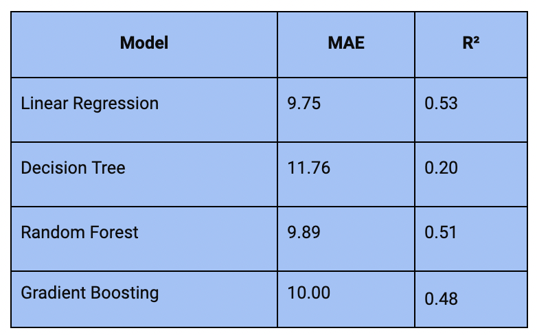
Linear Regression has the lowest MAE (9.75) and the highest R² (0.53), making it the best-performing model among those evaluated. It suggests that, despite its simplicity, Linear Regression is quite effective for this dataset.
Decision Tree Regressor shows the highest MAE (11.76) and the lowest R² (0.20), indicating it may be overfitting to the training data and performing poorly on the test data. On the other hand, Random Forest Regressor and Gradient Boosting Regressor have similar MAEs (9.89 and 10.00, respectively) and R² scores (0.51 and 0.48, respectively), performing slightly worse than the Linear Regression model but better than the Decision Tree.
Summary
So, this is how you can train and compare multiple Machine Learning models using Python. By comparing multiple models, we aim to select the most effective algorithm that offers the optimal balance of accuracy, complexity, and performance for their specific problem.
I hope you liked this article on how to compare multiple Machine Learning models. Feel free to ask valuable questions in the comments section below. You can follow me on Instagram for many more resources.