Classification on Imbalanced Data using Python
In Machine Learning, imbalanced data refers to a situation in classification problems where the number of observations in each class significantly differs. In such datasets, one class (the majority class) vastly outnumbers the other class (the minority class). This imbalance can lead to biased models that favour the majority class, resulting in poor predictive performance on the minority class, which is often the class of greater interest. So, if you want to learn how to perform classification on imbalanced data, this article is for you. In this article, I’ll take you through the task of performing classification on imbalanced data using Python.
Classification on Imbalanced Data: Process We Can Follow
Handling imbalanced data in classification tasks is a challenge that requires careful consideration of data preprocessing, resampling strategies, model choice, and evaluation metrics. Below is the process you can follow while performing classification on imbalanced datasets:
- Begin by analyzing the distribution of classes within your dataset to understand the extent of the imbalance.
- Determine the importance of each class in the context of your specific problem.
- Increase the number of instances in the minority class by replicating them to balance the class distribution.
- Some algorithms, like tree-based methods, are less sensitive to class imbalance. Consider using these or ensemble methods like Random Forest or Gradient Boosted Trees.
- Besides accuracy, use metrics that are informative for imbalanced datasets, such as Precision, Recall, F1 Score, or the Area Under the Receiver Operating Characteristic (AUROC) curve.
So, we need an imbalanced data for this task. I found an ideal dataset, which you can download from here.
Classification on Imbalanced Data using Python
Let’s get started with the task of performing classification on imbalanced data by importing the necessary Python libraries and the dataset:
import pandas as pd

# load the dataset
data = pd.read_csv("Insurance claims data.csv")

print(data.head())
policy_id subscription_length vehicle_age customer_age region_code \
0 POL045360 9.3 1.2 41 C8
1 POL016745 8.2 1.8 35 C2
2 POL007194 9.5 0.2 44 C8
3 POL018146 5.2 0.4 44 C10
4 POL049011 10.1 1.0 56 C13
region_density segment model fuel_type max_torque ... is_brake_assist \
0 8794 C2 M4 Diesel 250Nm@2750rpm ... Yes
1 27003 C1 M9 Diesel 200Nm@1750rpm ... No
2 8794 C2 M4 Diesel 250Nm@2750rpm ... Yes
3 73430 A M1 CNG 60Nm@3500rpm ... No
4 5410 B2 M5 Diesel 200Nm@3000rpm ... No
is_power_door_locks is_central_locking is_power_steering \
0 Yes Yes Yes
1 Yes Yes Yes
2 Yes Yes Yes
3 No No Yes
4 Yes Yes Yes
is_driver_seat_height_adjustable is_day_night_rear_view_mirror is_ecw \
0 Yes No Yes
1 Yes Yes Yes
2 Yes No Yes
3 No No No
4 No No Yes
is_speed_alert ncap_rating claim_status
0 Yes 3 0
1 Yes 4 0
2 Yes 3 0
3 Yes 0 0
4 Yes 5 0
[5 rows x 41 columns]
Let’s have a quick look at the column information and whether the data contains any null values or not:
data.info()<class 'pandas.core.frame.DataFrame'>
RangeIndex: 58592 entries, 0 to 58591
Data columns (total 41 columns):
# Column Non-Null Count Dtype
--- ------ -------------- -----
0 policy_id 58592 non-null object
1 subscription_length 58592 non-null float64
2 vehicle_age 58592 non-null float64
3 customer_age 58592 non-null int64
4 region_code 58592 non-null object
5 region_density 58592 non-null int64
6 segment 58592 non-null object
7 model 58592 non-null object
8 fuel_type 58592 non-null object
9 max_torque 58592 non-null object
10 max_power 58592 non-null object
11 engine_type 58592 non-null object
12 airbags 58592 non-null int64
13 is_esc 58592 non-null object
14 is_adjustable_steering 58592 non-null object
15 is_tpms 58592 non-null object
16 is_parking_sensors 58592 non-null object
17 is_parking_camera 58592 non-null object
18 rear_brakes_type 58592 non-null object
19 displacement 58592 non-null int64
20 cylinder 58592 non-null int64
21 transmission_type 58592 non-null object
22 steering_type 58592 non-null object
23 turning_radius 58592 non-null float64
24 length 58592 non-null int64
25 width 58592 non-null int64
26 gross_weight 58592 non-null int64
27 is_front_fog_lights 58592 non-null object
28 is_rear_window_wiper 58592 non-null object
29 is_rear_window_washer 58592 non-null object
30 is_rear_window_defogger 58592 non-null object
31 is_brake_assist 58592 non-null object
32 is_power_door_locks 58592 non-null object
33 is_central_locking 58592 non-null object
34 is_power_steering 58592 non-null object
35 is_driver_seat_height_adjustable 58592 non-null object
36 is_day_night_rear_view_mirror 58592 non-null object
37 is_ecw 58592 non-null object
38 is_speed_alert 58592 non-null object
39 ncap_rating 58592 non-null int64
40 claim_status 58592 non-null int64
dtypes: float64(3), int64(10), object(28)
memory usage: 18.3+ MB
data.isnull().sum()policy_id 0
subscription_length 0
vehicle_age 0
customer_age 0
region_code 0
region_density 0
segment 0
model 0
fuel_type 0
max_torque 0
max_power 0
engine_type 0
airbags 0
is_esc 0
is_adjustable_steering 0
is_tpms 0
is_parking_sensors 0
is_parking_camera 0
rear_brakes_type 0
displacement 0
cylinder 0
transmission_type 0
steering_type 0
turning_radius 0
length 0
width 0
gross_weight 0
is_front_fog_lights 0
is_rear_window_wiper 0
is_rear_window_washer 0
is_rear_window_defogger 0
is_brake_assist 0
is_power_door_locks 0
is_central_locking 0
is_power_steering 0
is_driver_seat_height_adjustable 0
is_day_night_rear_view_mirror 0
is_ecw 0
is_speed_alert 0
ncap_rating 0
claim_status 0
dtype: int64
The dataset contains 58,592 entries and 41 columns, including the target variable claim_status. It is based on the problem of insurance claim frequency prediction. Here’s a brief overview of some of the features:
- policy_id: Unique identifier for the insurance policy
- subscription_length, vehicle_age, customer_age: Numeric attributes related to the policy, vehicle, and customer
- region_code, segment, model, fuel_type: Categorical attributes representing the region, vehicle segment, model, and fuel type
- max_torque, max_power, engine_type: Specifications of the vehicle’s engine
- airbags, is_esc, is_adjustable_steering: Features related to the vehicle’s safety and convenience
- claim_status: Target variable indicating whether a claim was made (1) or not (0)
Next, I will perform exploratory data analysis to visualize and understand the distributions, relationships, and patterns in the data. It will include examining the distribution of the target variable and key features. Let’s start with visualizing the distribution of the claim_status to understand the class balance:
import matplotlib.pyplot as plt
import seaborn as sns
sns.set_style("whitegrid")

# plot the distribution of the target variable 'claim_status'
plt.figure(figsize=(8, 5))
sns.countplot(x='claim_status', data=data)
plt.title('Distribution of Claim Status')
plt.xlabel('Claim Status')
plt.ylabel('Count')
plt.show()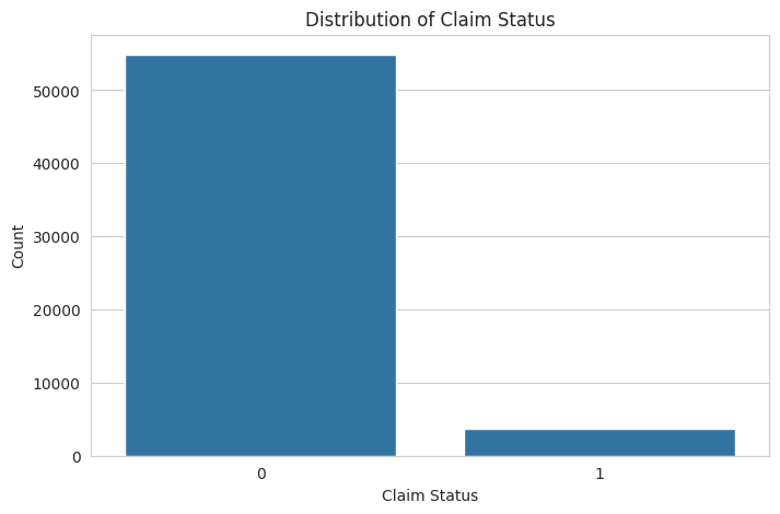
The distribution of the claim_status shows a significant imbalance between the classes, with much fewer claims (1) compared to no claims (0). This imbalance will be a challenge to address during the model training phase to ensure our model does not become biased toward predicting the majority class.
Next, I will perform an analysis of both numerical and categorical features to understand their distributions and relationships with the claim_status. Let’s start by examining the distributions of some key numerical features such as subscription_length, vehicle_age, and customer_age:
# selecting numerical columns for analysis
numerical_columns = ['subscription_length', 'vehicle_age', 'customer_age']

# plotting distributions of numerical features
plt.figure(figsize=(15, 5))
for i, column in enumerate(numerical_columns, 1):
    plt.subplot(1, 3, i)
    sns.histplot(data[column], bins=30, kde=True)
    plt.title(f'Distribution of {column}')

plt.tight_layout()
plt.show()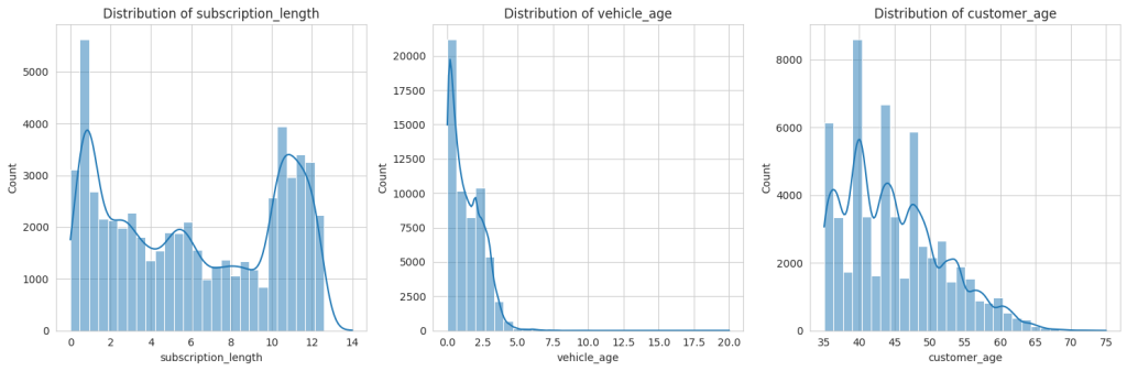
The distributions of the numerical features subscription_length, vehicle_age, and customer_age show the following characteristics:
- subscription_length: Most values are clustered around lower numbers, indicating that many policies have shorter subscription lengths.
- vehicle_age: This distribution is somewhat uniform but with spikes at specific ages, possibly representing common vehicle age intervals in the dataset.
- customer_age: This shows a fairly normal distribution, with the majority of customers falling within a middle-age range.
Next, we will analyze relevant categorical features to understand their variation and relationship with the claim_status. I’ll focus on features like region_code, segment, and fuel_type:
# selecting some relevant categorical columns for analysis
categorical_columns = ['region_code', 'segment', 'fuel_type']

# plotting distributions of categorical features
plt.figure(figsize=(15, 10))
for i, column in enumerate(categorical_columns, 1):
    plt.subplot(3, 1, i)
    sns.countplot(y=column, data=data, order = data[column].value_counts().index)
    plt.title(f'Distribution of {column}')
    plt.xlabel('Count')
    plt.ylabel(column)

plt.tight_layout()
plt.show()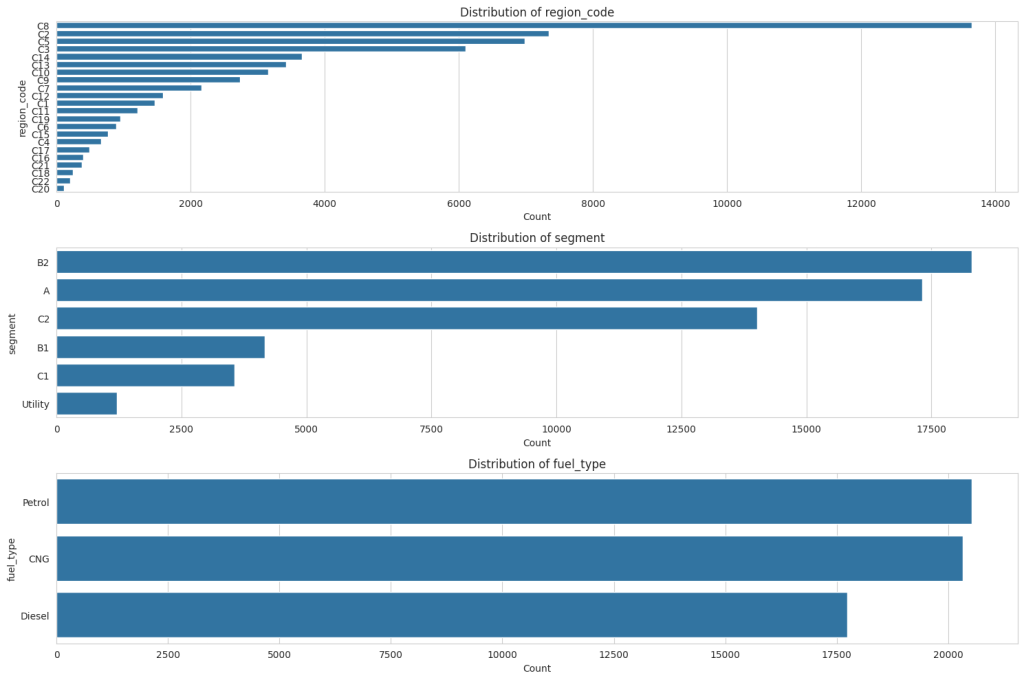
For ‘region_code,’ there is a wide variety of codes, each with varying counts, but a few specific codes dominate with much higher counts than others. In the ‘segment’ distribution, there are fewer categories, with the ‘B2’ segment being the most common, followed by ‘A’ and ‘C2,’ and the ‘Utility’ segment being the least common. Lastly, ‘fuel_type’ shows three categories: ‘Petrol’ has the highest count than CNG and Diesel.
Handling Class Imbalance
The next step is to balance the dataset using oversampling to handle the class imbalance observed in the claim_status. Let’s proceed with balancing the classes:
from sklearn.utils import resample

# separate majority and minority classes
majority = data[data.claim_status == 0]
minority = data[data.claim_status == 1]

# oversample the minority class
minority_oversampled = resample(minority,
                                replace=True,
                                n_samples=len(majority),
                                random_state=42)

# combine majority class with oversampled minority class
oversampled_data = pd.concat([majority, minority_oversampled])

# check the distribution of undersampled and oversampled datasets
oversampled_distribution = oversampled_data.claim_status.value_counts()

oversampled_distribution
0 54844
1 54844
Name: claim_status, dtype: int64
After performing oversampling on the minority class, both classes are balanced with 54,844 entries each. Now, let’s have a look at some key variables to see what the balanced data looks like:
# plotting the distribution of 'customer_age', 'vehicle_age', and 'subscription_length' with respect to 'claim_status'
plt.figure(figsize=(15, 5))

# 'customer_age' distribution
plt.subplot(1, 3, 1)
sns.histplot(data=oversampled_data, x='customer_age', hue='claim_status', element='step', bins=30)
plt.title('Customer Age Distribution')

# 'vehicle_age' distribution
plt.subplot(1, 3, 2)
sns.histplot(data=oversampled_data, x='vehicle_age', hue='claim_status', element='step', bins=30)
plt.title('Vehicle Age Distribution')

# 'subscription_length' distribution
plt.subplot(1, 3, 3)
sns.histplot(data=oversampled_data, x='subscription_length', hue='claim_status', element='step', bins=30)
plt.title('Subscription Length Distribution')

plt.tight_layout()
plt.show()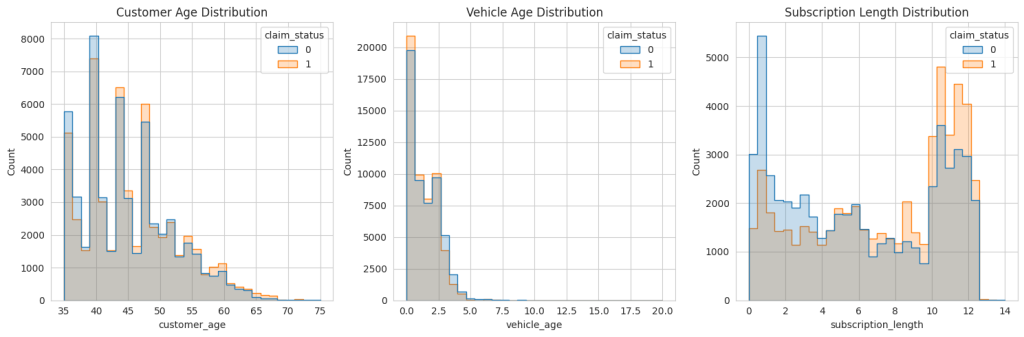
The oversampled data does look like the original data. So, let’s move forward.
Feature Selection
Now, we will identify the most important variables for predicting insurance frequency claims. It involves analyzing both categorical and numerical features to determine their impact on the target variable. We will use feature importance techniques suitable for both types of variables. Let’s start with feature selection to identify the most important variables:
from sklearn.ensemble import RandomForestClassifier
from sklearn.preprocessing import LabelEncoder

# encode categorical variables
le = LabelEncoder()
encoded_data = data.apply(lambda col: le.fit_transform(col) if col.dtype == 'object' else col)

# separate features and target variable
X = encoded_data.drop('claim_status', axis=1)
y = encoded_data['claim_status']

# create a random forest classifier model
rf_model = RandomForestClassifier(random_state=42)
rf_model.fit(X, y)

# get feature importance
feature_importance = rf_model.feature_importances_

# create a dataframe for visualization of feature importance
features_df = pd.DataFrame({'Feature': X.columns, 'Importance': feature_importance})
features_df = features_df.sort_values(by='Importance', ascending=False)

print(features_df.head(10))  # displaying the top 10 important features
Feature Importance
0 policy_id 0.321072
1 subscription_length 0.248309
3 customer_age 0.176639
2 vehicle_age 0.135190
5 region_density 0.053838
4 region_code 0.052649
7 model 0.000957
24 length 0.000846
26 gross_weight 0.000834
11 engine_type 0.000791
The top 10 most important variables for predicting insurance frequency claims, according to the Random Forest model, are:
- policy_id: Unique identifier for the insurance policy
- subscription_length: Length of the insurance subscription
- customer_age: Age of the customer
- vehicle_age: Age of the vehicle
- region_density: Population density of the region
- region_code: Code representing the region
- model: Model of the vehicle
- engine_type: Type of engine in the vehicle
- gross_weight: Gross weight of the vehicle
- length: Length of the vehicle
These variables appear to have the most influence on the likelihood of an insurance claim being made. However, it’s notable that policy_id has a very high importance, which might not be intuitively relevant for prediction. So, we need to make sure to drop the policy_id column while model training.
Model Training
The next step is to build a predictive model using the oversampled data. Given the nature of the task (binary classification), a suitable algorithm could be logistic regression, random forest, or gradient boosting. Considering the effectiveness of random forests in handling both numerical and categorical data and their ability to model complex interactions, we’ll proceed with a Random Forest classifier:
from sklearn.model_selection import train_test_split
from sklearn.metrics import classification_report, accuracy_score
from sklearn.ensemble import RandomForestClassifier

# drop 'Policy_id' column from the data
oversampled_data = oversampled_data.drop('policy_id', axis=1)

# prepare the oversampled data
X_oversampled = oversampled_data.drop('claim_status', axis=1)
y_oversampled = oversampled_data['claim_status']

# encoding categorical columns
X_oversampled_encoded = X_oversampled.apply(lambda col: LabelEncoder().fit_transform(col) if col.dtype == 'object' else col)

# splitting the dataset into training and testing sets
X_train, X_test, y_train, y_test = train_test_split(
    X_oversampled_encoded, y_oversampled, test_size=0.3, random_state=42)

# create and train the Random Forest model
rf_model_oversampled = RandomForestClassifier(random_state=42)
rf_model_oversampled.fit(X_train, y_train)

# predictions
y_pred = rf_model_oversampled.predict(X_test)

print(classification_report(y_test, y_pred))
precision recall f1-score support
0 1.00 0.98 0.99 16574
1 0.98 1.00 0.99 16333
accuracy 0.99 32907
macro avg 0.99 0.99 0.99 32907
weighted avg 0.99 0.99 0.99 32907
The classification report above provides various metrics to evaluate the performance of the predictive model on the test data. Here’s an interpretation of the results:
- For class 0 (no claim), precision is 1.00, meaning that when the model predicts no claim, it is correct 100% of the time. For class 1 (claim), precision is 0.98, indicating that when the model predicts a claim, it is correct 98% of the time.
- For class 0, recall is 0.98, signifying that the model correctly identifies 98% of all actual no-claim instances. For class 1, recall is 1.00, showing that the model correctly identifies 100% of all actual claim instances.
- The F1-score for both classes is 0.99, indicating a high balance between precision and recall. It means the model is both accurate and reliable in its predictions across both classes.
- The overall accuracy of the model is 99%, which means that it correctly predicts the claim status for 99% of the cases in the test dataset.
- The macro average for precision, recall and F1-score is 0.99, reflecting the average performance of the model across both classes without considering the imbalance in class distribution. This high value suggests that the model performs well across both classes. The weighted average for precision, recall, and F1-score is also 0.99, taking into account the imbalance in class distribution. It indicates that, on average, the model performs consistently well across the different classes when considering their distribution in the dataset.
These results indicate a highly effective model for predicting insurance claims, with strong performance metrics across both classes of outcomes. The high recall for claims (class 1) is particularly notable as it implies that the model is very effective at identifying the instances where claims occur, which is often the primary concern in imbalanced datasets.
Now, let’s label the original imbalanced data using our model to see how many instances are correctly classified from our model:
original_encoded = data.drop('policy_id', axis=1).copy()
encoders = {col: LabelEncoder().fit(X_oversampled[col]) for col in X_oversampled.select_dtypes(include=['object']).columns}

for col in original_encoded.select_dtypes(include=['object']).columns:
    if col in encoders:
        original_encoded[col] = encoders[col].transform(original_encoded[col])

original_encoded_predictions = rf_model_oversampled.predict(original_encoded.drop('claim_status', axis=1))

comparison_df = pd.DataFrame({
    'Actual': original_encoded['claim_status'],
    'Predicted': original_encoded_predictions
})

print(comparison_df.head(10))
Actual Predicted
0 0 0
1 0 0
2 0 0
3 0 0
4 0 0
5 0 0
6 0 0
7 0 0
8 0 0
9 0 0
Let’s visualize the percentage of correctly classified and misclassified samples:
correctly_classified = (comparison_df['Actual'] == comparison_df['Predicted']).sum()
incorrectly_classified = (comparison_df['Actual'] != comparison_df['Predicted']).sum()

classification_counts = [correctly_classified, incorrectly_classified]
labels = ['Correctly Classified', 'Misclassified']

# create a pie chart
plt.figure(figsize=(8, 8))
plt.pie(classification_counts, labels=labels, autopct='%1.1f%%', startangle=140, colors=['#4CAF50', '#FF5733'])
plt.title('Classification Accuracy')
plt.show()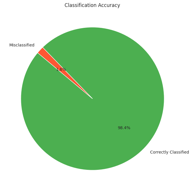
So, we can see that our model performs well on the original imbalanced data as well.
Summary
So, this is how to handle class imbalance and perform classification on imbalanced data. Imbalanced data refers to a situation in classification problems where the number of observations in each class significantly differs. In such datasets, one class (the majority class) vastly outnumbers the other class (the minority class). This imbalance can lead to biased models that favour the majority class, resulting in poor predictive performance on the minority class, which is often the class of greater interest.